Introduction

My first post is going to be trivial but, I think, quite mesmerizing.

I avidly follow a website called R-Bloggers, a content aggregator where you can find daily updates of a huge variety of blogs treating a plethora of topics. I learned that, thanks to the power of R, I could be able to accomplish everything I deem important in life: creating memes, making pixel art, and generate sCATterplots. On a slightly more serious note, I discovered extremely interesting blogs, like Variance Explained, and useful R packages, for example sjPlot.

Clifford attractors

Recently, I stumbled upon this blog post showing how to draw Clifford A. Pickover’s strange attractors in R. They are defined by the following equations:

\[ x_{n+1} = sin( \textbf{a} y_{n} ) + \textbf{c} cos( \textbf{a} x_{n} ) \]
\[ y_{n+1} = sin( \textbf{b} x_{n} ) + \textbf{d} cos( \textbf{b} y_{n} ) \]

The free parameters (in bold) define each attractor. When using \(\textbf{a}\) = 1.5, \(\textbf{b}\) = -1.8, \(\textbf{c}\) = 1.6, and \(\textbf{d}\) = 0.9 – sequentially through 1,000,000¹ steps – the result looks like this:

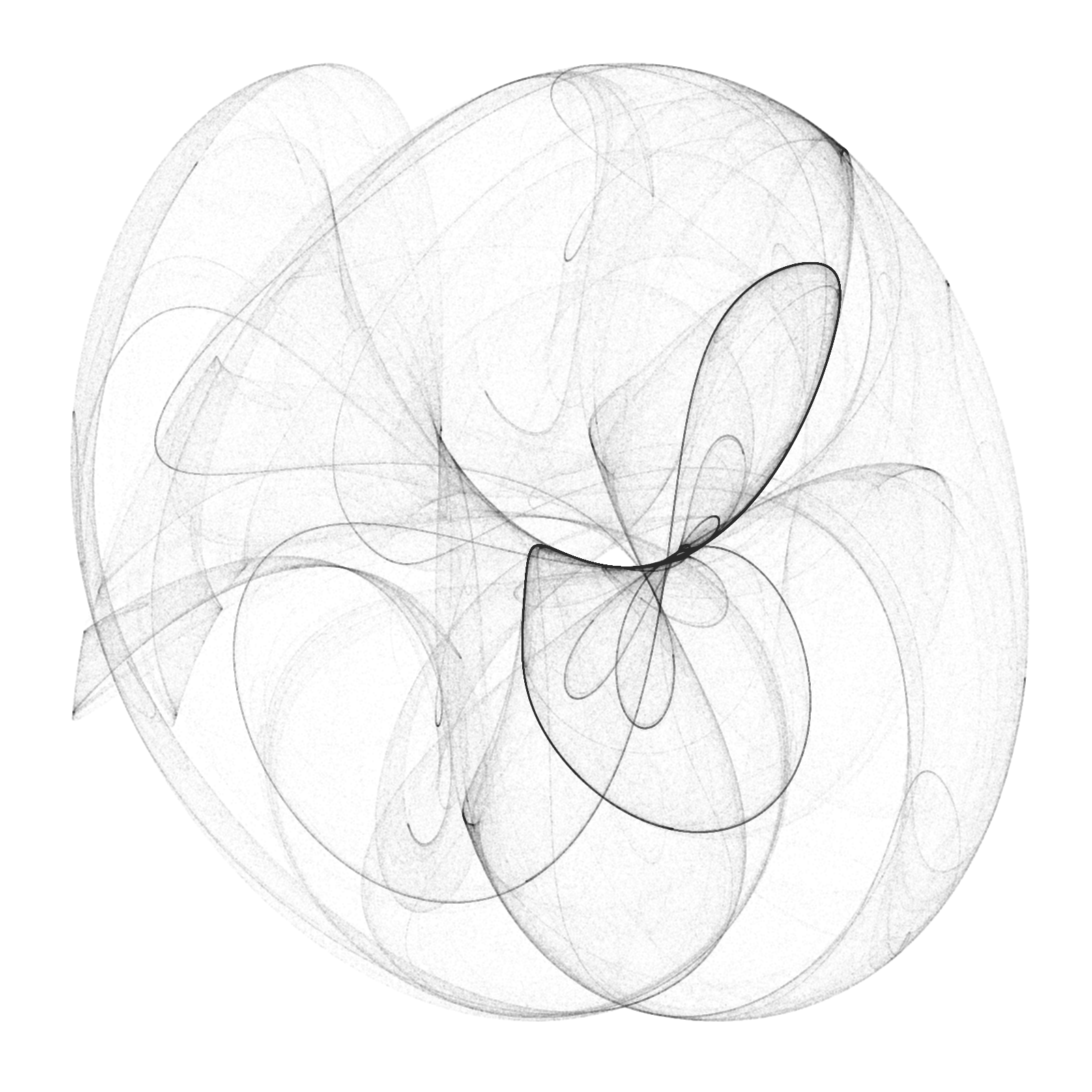
Figure 1. My first Clifford attractor.

This is sweet, but something is missing… perhaps there are not enough points. Let’s use 10,000,000!

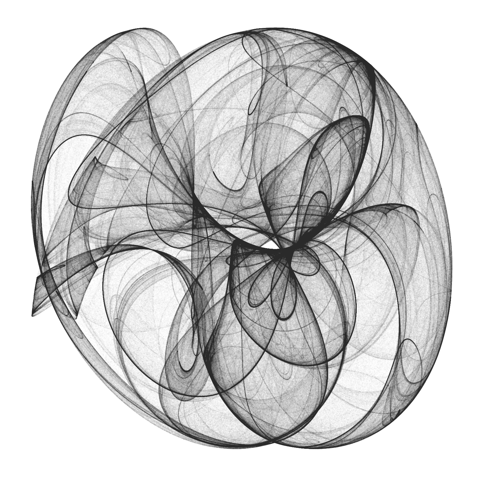
Figure 2. A nice-looking Clifford attractor.

That’s more like it. Now let’s make another attractor, using 10,000,000 magenta points.

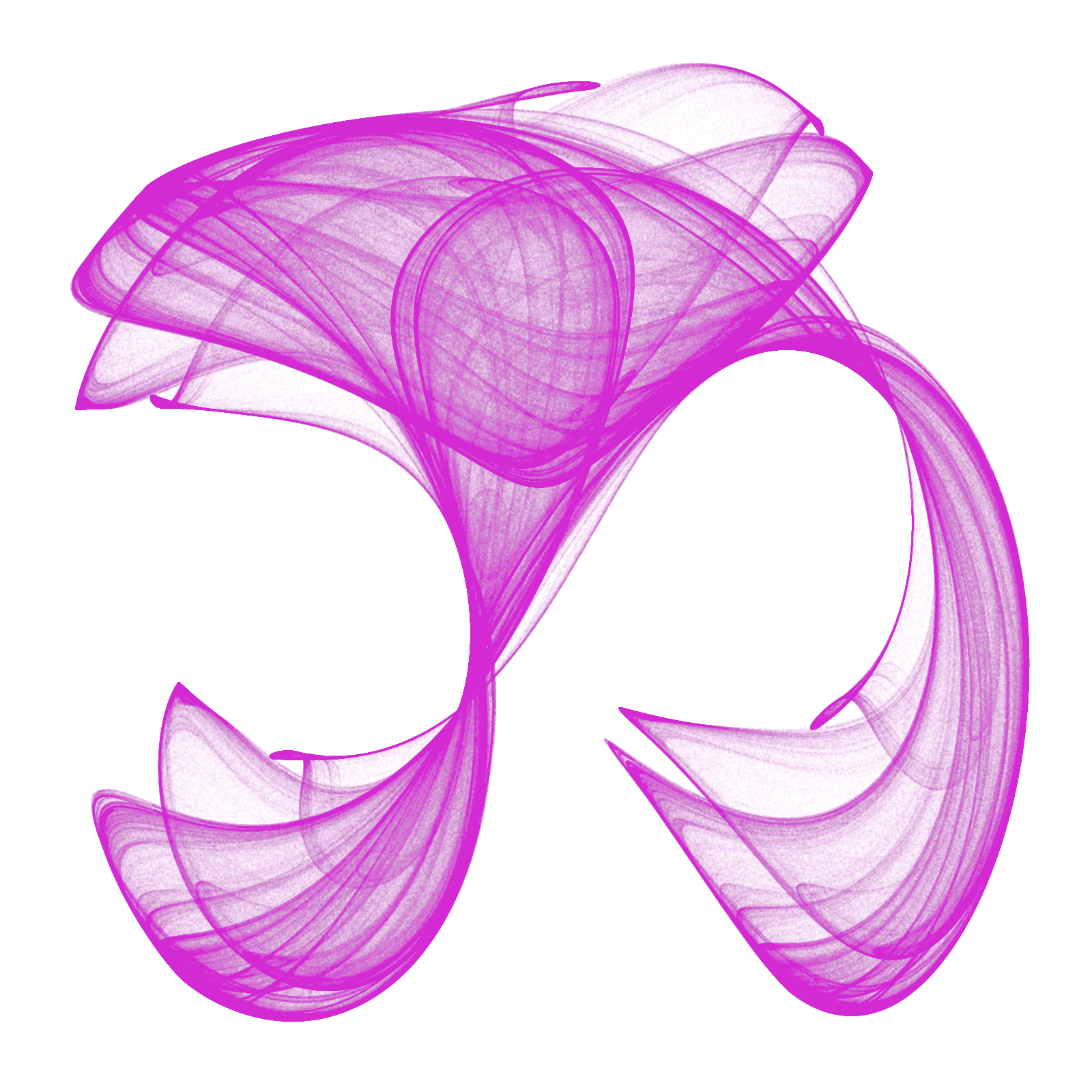
Figure 3. A magenta Clifford attractor.

Oh yeah, that’s juicy².

I’ve got an idea: let’s make a few more, and then overlay them!

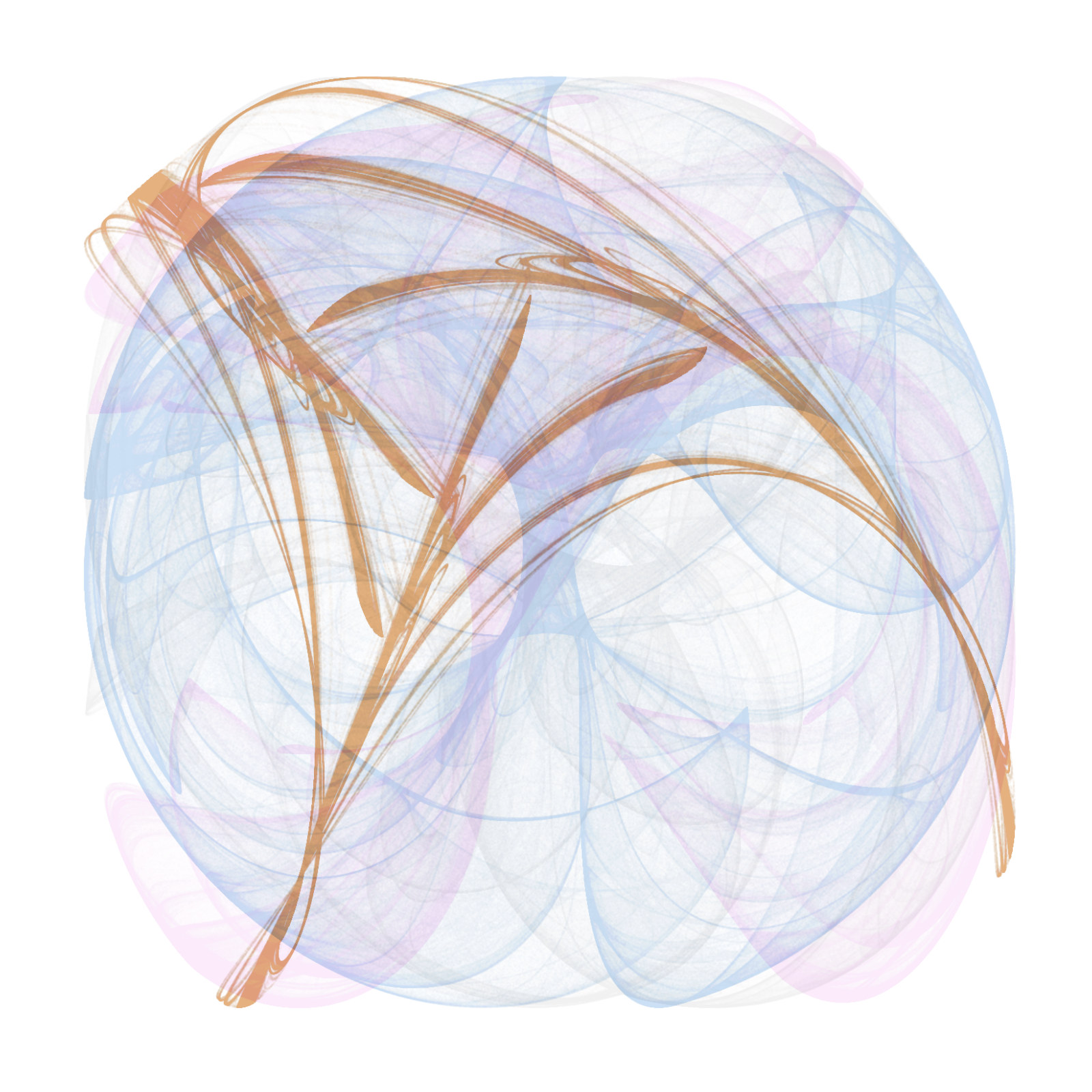
Figure 4. Black, magenta, blue, and golden Clifford attractors.

Fantastic. This took a long time but… totally worth the effort!

In case you want to waste countless hours hunting for the perfect Clifford attractor, here is the code:

##### CREATE A CLIFFORD ATTRACTOR #####

# load packages
library(Rcpp)
library(ggplot2)
library(png)

# custom ggplot2 minimalist theme
opt <- theme(
  legend.position = "none",
  panel.background = element_rect(fill = "white"),
  axis.ticks = element_blank(),
  panel.grid = element_blank(),
  axis.title = element_blank(),
  axis.text = element_blank()
)

# function drawing the position of each point (starting from positions x and y) using Pickover's equations
cppFunction('DataFrame createTrajectory(int n, double x0, double y0, 
            double a, double b, double c, double d) {
            // create the columns
            NumericVector x(n);
            NumericVector y(n);
            x[0]=x0;
            y[0]=y0;
            for(int i = 1; i < n; ++i) {
            x[i] = sin(a*y[i-1])+c*cos(a*x[i-1]);
            y[i] = sin(b*x[i-1])+d*cos(b*y[i-1]);
            }
            // return a new data frame
            return DataFrame::create(_["x"]= x, _["y"]= y);
            }
            ')

# assign values to free parameters
# black attractor
a <- 1.5
b <- -1.8
c <- 1.6
d <- 0.9
# # magenta attractor
# a <- -1.4
# b <- 1.6
# c <- 1.0
# d <- 0.7
# # blue attractor
# a <- -1.8
# b <- 1.8
# c <- 0.9
# d <- 0.7
# # gold attractor
# a <- -1.2
# b <- 1.7
# c <- 0.9
# d <- 0.6

df <- createTrajectory(10000000, 0, 0, a, b, c, d) # calculate the coordinates of 10,000,000 points (starting from position [x = 0, y = 0]
attractor <- ggplot(df, aes(x, y)) +
  geom_point(color = "black", shape = 46, alpha = .01) +
  opt # create the graph
# magenta attractor: color="#e017e0"
# blue attractor: color="#2570da"
# gold attractor: color="#cd7f32"

# save as .png
png("attractor.png", units = "px", width = 1600, height = 1600, res = 300)
attractor
dev.off() # close device

##### OVERLAY ATTRACTORS #####

# load packages
library(grid)
library(gridExtra)

# assuming attractors are saved in separate .png files...
# load images
attractor.black <- readPNG("attractor_black.png")
attractor.mag <- readPNG("attractor_mag.png")
attractor.blue <- readPNG("attractor_blue.png")
attractor.gold <- readPNG("attractor_gold.png")

# convert to raster
# (play with the alpha levels to modify transparency)
attractor.black.raster <- matrix(rgb(attractor.black[, , 1], attractor.black[, , 2], attractor.black[, , 3], alpha = 1), nrow = dim(attractor.black)[1])
attractor.mag.raster <- matrix(rgb(attractor.mag[, , 1], attractor.mag[, , 2], attractor.mag[, , 3], alpha = .6), nrow = dim(attractor.mag)[1])
attractor.blue.raster <- matrix(rgb(attractor.blue[, , 1], attractor.blue[, , 2], attractor.blue[, , 3], alpha = .6), nrow = dim(attractor.blue)[1])
attractor.gold.raster <- matrix(rgb(attractor.gold[, , 1], attractor.gold[, , 2], attractor.gold[, , 3], alpha = .6), nrow = dim(attractor.gold)[1])

# overlay all images as different static annotations in a ggplot2 object
overlay <- ggplot(data.frame()) +
  annotation_custom(rasterGrob(attractor.black.raster)) +
  annotation_custom(rasterGrob(attractor.mag.raster)) +
  annotation_custom(rasterGrob(attractor.blue.raster)) +
  annotation_custom(rasterGrob(attractor.gold.raster)) +
  opt

# save as .png
png("overlay.png", units = "px", width = 1600, height = 1600, res = 300)
overlay
dev.off()
dev.off()